This guide demonstrates how to lock cells in Excel worksheets to protect formulas or other data from being changed, while allowing selected cells to remain unlocked. This is useful to prevent accidental changes to the worksheet and to enhance navigability by allowing users to select only the modifiable cells. The information in this guide was tested on a Windows XP system using Microsoft Excel ver. 2003. The steps in this guide should be similar for other versions of Excel. An example worksheet provided for this guide is provided here.
Steps to Protect Excel Worksheets
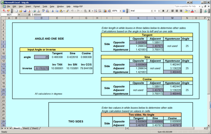
1. Use the Control or Shift key to select individual cells that are to remain unprotected and modifiable by the user. The screenshot below shows the selected cells in grey. All unselected cells will be protected.
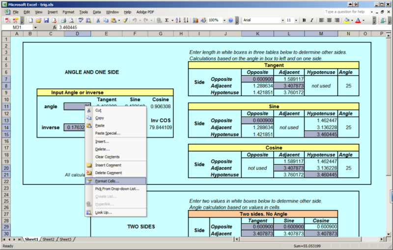
2. Right-click over one of the selected cells and select Format Cells… from the right-click menu.
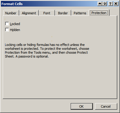
3. In the Format Cell dialog that appears, select the Protection Tab and unselect both the Locked and Hidden options and then click OK.
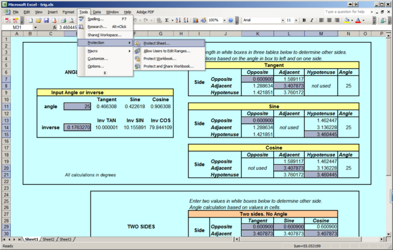
4. From the application menu, select Tools->Protection->Protect Sheet…
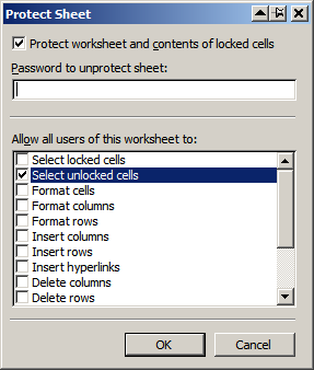
5. In the Protect Sheet Dialog that appears, ensure that Protect worksheet and contents of locked cells a the top and Select unlocked cells from the list are selected and then hit OK.
That’s all there is to it. The Tab key can be used to move between the selectable cells. All other cells are protected. To make changes to the worksheet, select Tools->Protection->Unprotect Sheet…


